I use Excel a lot, always have done and probably always will do. I find it a great tool for estimating, quick planning and most of all quick analysis. Over the years I have learnt a few tips and tricks that have sped up the way I use of Excel.
Often, I come across others who do not know these tips and tricks. They may not work for everyone in every scenario but hopefully they will help some people some of the time.
Tables
Most of the time the content that I work with in Excel is best thought of as a table and conveniently, there is an option to work with the content as a table. The biggest benefit of tables is the ability to reference the content regardless of the location of the table.
Format as Table
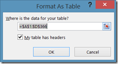
The first step is to highlight the content that will make up the table and then to click the Format as Table option in the Home ribbon:
Once clicked, you get the option to select a design. The design can be changed later.
The next prompt confirms the area to be turned into a table and also confirms whether the selected area includes headers. In 90% of cases, I find that the content does, or should contain headers as I use them in calculations.
After clicking on OK the table has been created, it has formatting and it also has filters by default.
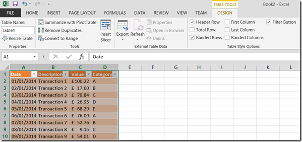
Table Configuration
Table Name
Once the table has been created, it is important to give it a sensible name:
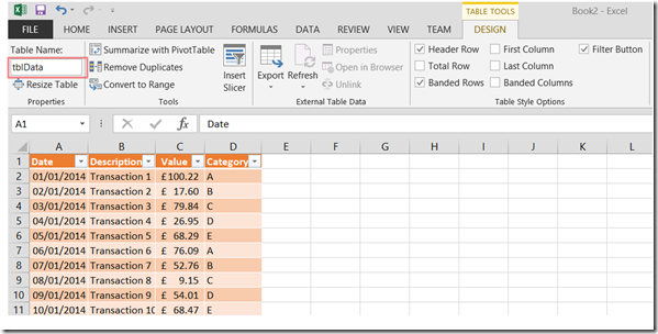
I usually prefix the tables with tbl as it makes it easy to reference in formulae.
Table Style
The style of the table can be changed at this stage too:
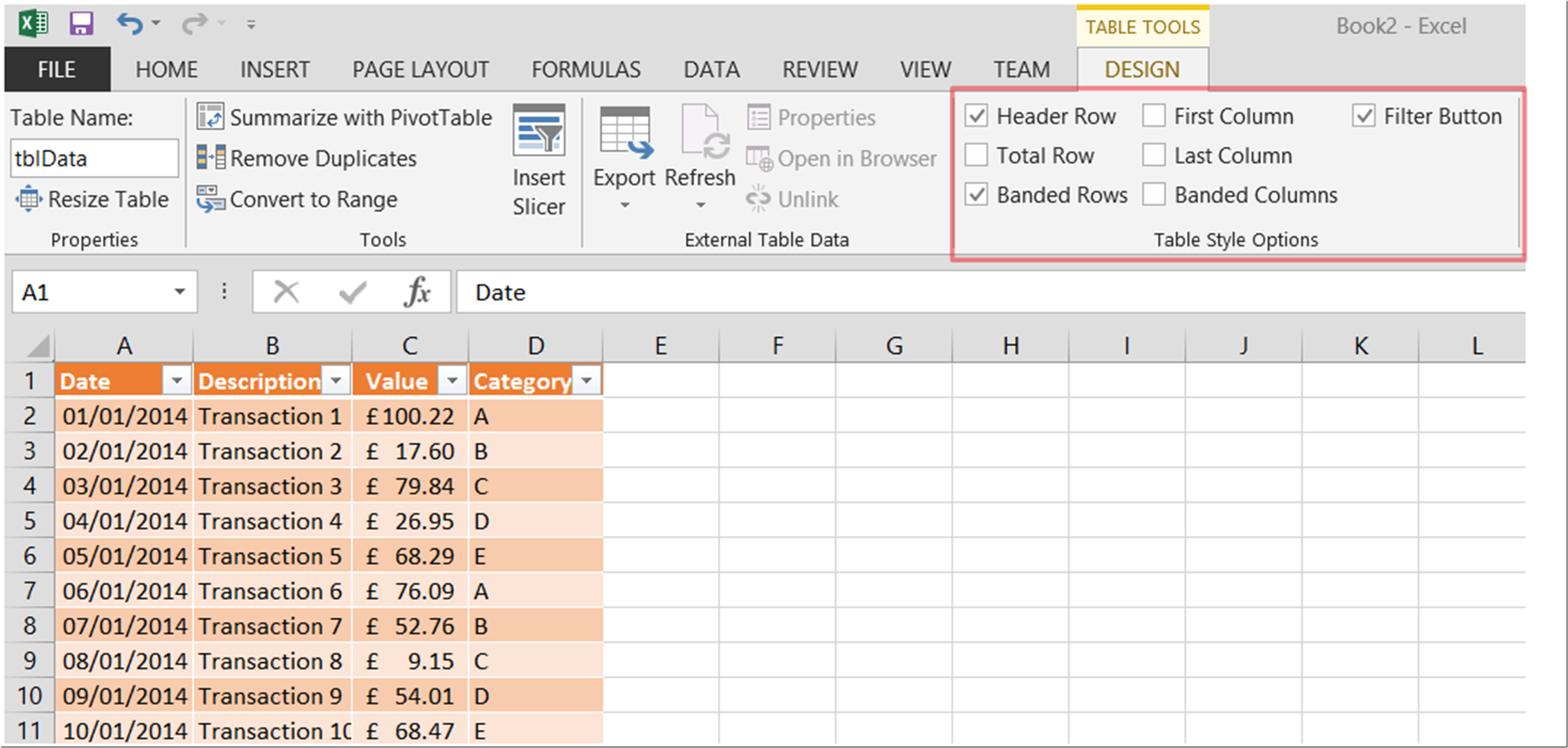
Using the checkboxes, there is a lot that can be done to configure the table:
| Header Row | Sets the first row in the table as a header row meaning it is formatted differently and can be referenced in formulae |
| Total Row | Sets the last row in the table as a total row meaning it is formatted differently and has a choice of built in formulae to act upon the column |
| Banded Rows | Applies alternating formatting for all rows except Header and Total rows |
| First Column | Formats the first column in the same style as the Header row |
| Last Column | Formats the last column in the same style as the Header row |
| Banded Columns | Applies alternating formatting for all columns |
| Filter Button | Applies the filter drop-down in the Header row |
Table References
Now that a table has been defined with the name of tblData it can be referenced using the following syntax:
| Syntax | Example |
|---|---|
| tableName[columnName] | SUM(tblData[Value]) will give the SUM of the Value column in the tblData table |
| [@[columnName]] | Used to refer to a column when within a table |
| tableName[[#Totals],[columnName]] | tblData[[#Totals],[Value]] will give the #Totals value of
the Value column in the tblData table. Note that the #Totals value will be the calculation selected in the table and not automatically a SUM of the values |
There are many other examples of how to reference the values of a table at the following location:
Formulae
Now that there is a table and the content can be referenced, analysis of the table can take place easily.
SUMIF, COUNTIF, AVERAGEIF
This set of functions work in the same way, with the same syntax:
=SUMIF(range, criteria, [, sum_range])
where the inputs are as follows:
| Input | Definition |
|---|---|
| range | Range is the set of cells that will be evaluated to see if they match the criteria |
| criteria | The value that the range is evaluated against |
| sum_range | This is an optional input that defines the values to be added together |
In the following example a calculation is being carried out against a table:
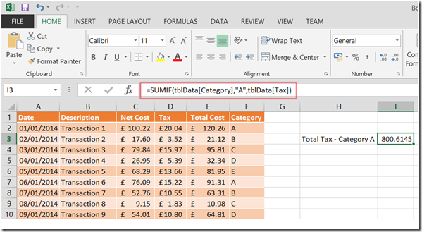
The following formula is being used:
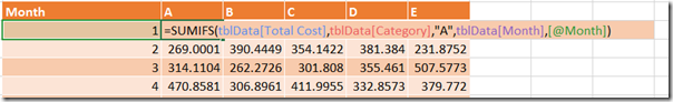
=SUMIF(tblData[Category],"A",tblData[Tax])
The result of the formula is the SUM of the Tax column of table tblData where each value of the Category column is equal to A.
That is all well and good, but what if you wanted to add a condition to the evaluation of the range?
Well, the criteria element can contain conditions:
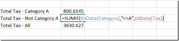
The previous example show the use of "<>A" for the criteria. Other options include:
| Syntax | Use |
|---|---|
| "=*A*" | Contains A |
| "=A*" | Starts with A |
| "=*A" | Ends with A |
| "=A?B" | ? represents any character |
For more information on these formulae see the following pages:
SUMIFS, COUNTIFS, AVERAGEIFS
This family of functions extends the number of criteria that can be evaluated but the syntax is different:
=SUMIFS(sum_range, criteria_range1, criteria1, [, criteria_range2, criteria2])
where the inputs are as follows:
| Input | Definition |
|---|---|
| sum_range | This defines the values to be added together |
| criteria_range1 | The range is the set of cells that will be evaluated to see if they match the criteria1 |
| criteria1 | The value that the criteria_range1 is evaluated against |
| criteria_range2 | The range is the set of cells that will be evaluated to see if they match the criteria2 |
| criteria2 | The value that the criteria_range2 is evaluated against |
Additional sets of ranges and criteria can be added as required.
In the following example a calculation is being carried out against a table:
Summary
The use of tables to reference data and the SUM and SUMIF families of functions are incredibly useful tools when it comes to collating and analysing data. That is not to say they are the only tools, nor to say that they are perfect. There are some shortcomings however in most cases they are a very useful starting point.